
This excerpt is from an article by Nilson Souto originally published on Toptal.
Physics simulation is a field within computer science that aims to reproduce physical phenomena using a computer. In general, these simulations apply numerical methods to existing theories to obtain results that are as close as possible to what we observe in the real world. This allows us, as advanced game developers, to predict and carefully analyze how something would behave before actually building it, which is almost always simpler and cheaper to do.
The range of applications of physics simulations is enormous. The earliest computers were already being used to perform physics simulations – for example, to predict the ballistic motion of projectiles in the military. It is also an essential tool in civil and automotive engineering, illuminating how certain structures would behave in events like an earthquake or a car crash. And it doesn’t stop there. We can simulate things like astrophysics, relativity, and lots of other insane stuff we are able to observe in among the wonders of nature.
Simulating physics in video games is very common, since most games are inspired by things we have in the real world. Many games rely entirely on the physics simulation to be fun. That means these games require a stable simulation that will not break or slow down, and this is usually not trivial to achieve.
In any game, only certain physical effects are of interest. Rigid body dynamics – the movement and interaction of solid, inflexible objects—is by far the most popular kind of effect simulated in games. That’s because most of the objects we interact with in real life are fairly rigid, and simulating rigid bodies is relatively simple (although as we will see, that doesn’t mean it’s a cakewalk). A few other games require the simulation of more complicated entities though, such as deformable bodies, fluids, magnetic objects, etc..
In this video game physics tutorial series, rigid body simulation will be explored, starting with simple rigid body motion in this article, and then covering interactions among bodies through collisions and constraints in the following installments. The most common equations used in modern game physics engines such as Box2D, Bullet Physics and Chipmunk Physics will be presented and explained.
Rigid Body Dynamics
In video game physics, we want to animate objects on screen and give them realistic physical behavior. This is achieved with physics-based procedural animation, which is animation produced by numerical computations applied to the theoretical laws of physics.
Animations are produced by displaying a sequence of images in succession, with objects moving slightly from one image to the next. When the images are displayed in quick succession, the effect is an apparent smooth and continuous movement of the objects. Thus, to animate the objects in a physics simulation, we need to update the physical state of the objects (e.g. position and orientation), according to the laws of physics multiple times per second, and redraw the screen after each update.
The physics engine is the software component that performs the physics simulation. It receives a specification of the bodies that are going to be simulated, plus some configuration parameters, and then the simulation can be stepped. Each step moves the simulation forward by a few fractions of a second, and the results can be displayed on screen afterwards. Note that physics engines only perform the numerical simulation. What is done with the results may depend on the requirements of the game. It is not always the case that the results of every step wants to be drawn to the screen.
The motion of rigid bodies can be modeled using newtonian mechanics, which is founded upon Isaac Newton’s famous Three Laws of Motion:
- Inertia: If no force is applied on an object, its velocity (speed and direction of motion) shall not change.
- Force, Mass, and Acceleration: The force acting on an object is equal to the mass of the object multiplied by its acceleration (rate of change of velocity). This is given by the formula F = ma.
- Action and Reaction: “For every action there is an equal and opposite reaction.” In other words, whenever one body exerts a force on another, the second body exerts a force of the same magnitude and opposite direction on the first.
Based on these three laws, we can make a physics engine that is able to reproduce the dynamic behavior we’re so familiar with, and thus create an immersive experience for the player.
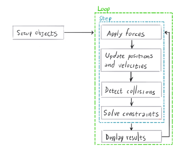
The following diagram shows a high level overview of the general procedure of a physics engine:
Vectors
In order to understand how physics simulations work, it is crucial to have a basic understanding of vectors and their operations. If you are already familiar with vector math, read on. But if you are not, or you want to brush up, take a minute to review the appendix at the end of this article.
Particle Simulation
A good stepping stone to understanding rigid body simulation is to start with particles. Simulating particles is simpler than simulating rigid bodies, and we can simulate the latter using the same principles, but adding volume and shape to the particles.
A particle is just a point in space that has a position vector, a velocity vector and a mass. According to Newton’s First Law, its velocity will only change when a force is applied on it. When its velocity vector has a non-zero length, its position will change over time.
To simulate a particle system, we need to first create an array of particles with an initial state. Each particle must have a fixed mass, an initial position in space and an initial velocity. Then we have to start the main loop of the simulation where, for each particle, we have to compute the force that is currently acting on it, update its velocity from the acceleration produced by the force, and then update its position based on the velocity we just computed.
The force may come from different sources depending on the kind of simulation. It can be gravity, wind, or magnetism, among others – or it can be a combination of these. It can be a global force, such as constant gravity, or it can be a force between particles, such as attraction or repulsion.
To make the simulation run at a realistic pace, the time step we “simulate” should be the same as the real amount of time that passed since the last simulation step. However, this time step can be scaled up to make the simulation run faster, or scaled down to make it run in slow motion.
Suppose we have one particle with mass m, position p(ti) and velocity v(ti) at an instant of time ti. A force f(ti)is applied on that particle at that time. The position and velocity of this particle at a future time ti + 1, p(ti + 1)and v(ti + 1) respectively, can be computed with:
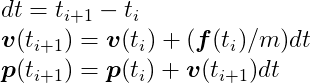
In technical terms, what we’re doing here is numerically integrating an ordinary differential equation of motion of a particle using the semi-implicit Euler method, which is the method most game physics engines use due to its simplicity and acceptable accuracy for small values of the time span, dt. The Differential Equation Basics lecture notes from the amazing Physically Based Modeling: Principles and Practice course, by Drs. Andy Witkin and David Baraff, is a nice article to get a deeper look into the numerical methodology of this method.
Interested in getting into the nitty-gritty parts of physics mathematics and programming? Check out Nilson Souto’s complete series on Toptal!